Introduction :
In the ever-changing landscape of data analytics, the ARIMA (AutoRegressive Integrated Moving Average) forecasting model emerges as a powerful tool for predicting future trends and patterns. As businesses strive to stay ahead in dynamic markets, leveraging the capabilities of ARIMA becomes vital for making informed decisions and gaining a competitive edge. In this comprehensive guide, we will delve deep into the intricacies of the ARIMA forecasting model, shedding light on its applications across various industries and its significance in time series analysis.
Table of Contents
1. ARIMA Forecasting Model:
The ARIMA model, a statistical method for analyzing and forecasting time series data, combines three essential components: autoregression, differencing, and moving averages. By understanding the patterns and dependencies within the data, ARIMA enables accurate prediction of future values.
2. Understanding Time Series Analysis:
What is Time Series Data?
Time series data consists of observations collected sequentially over time. Analyzing time series data aims to uncover underlying patterns, trends, and seasonality to gain insights into the data’s behavior.
Importance of Time Series Analysis:
Time plays a crucial role in decision-making across industries. Time series analysis, especially utilizing the ARIMA forecasting model, allows us to analyze and exploit temporal patterns, aiding in more informed decision-making processes.
3. Basics of ARIMA Forecasting Model:
The ARIMA model comprises three main components:
a. Autoregressive (AR) Component:
The AR component represents the relationship between the current observation and a certain number of lagged observations from previous time steps, allowing us to capture dependencies within the data.
b. Integrated (I) Component:
The integrated component involves differencing the raw observations to achieve stationarity, ensuring that the mean, variance, and covariance remain constant over time.
c. Moving Average (MA) Component:
The MA component captures the relationship between the current observation and the residual errors derived from a moving average model applied to lagged observations.
4. Advantages of ARIMA Forecasting Model:
a. Flexibility to handle various types of time series data.
b. Ability to capture both linear and non-linear relationships.
c. Robustness against outliers and irregularities in the data.
d. Interpretability of model parameters.
5. Applications of ARIMA Forecasting Model:
ARIMA finds extensive applications across diverse domains, including:
a. Financial Forecasting:
ARIMA aids stock market analysis, risk management, and predicting financial market trends.
b. Demand Forecasting:
Retailers leverage ARIMA to forecast product demand, optimize inventory management, and enhance supply chain efficiency.
c. Weather Forecasting:
Meteorologists utilize ARIMA to predict weather patterns, such as rainfall, temperature, precipitation, and wind speed, based on historical climate data.
6. Steps to Build an ARIMA Forecasting Model:
a. Data Collection and Preprocessing:
Gather historical data relevant to the phenomenon under study and preprocess it to ensure consistency and quality.
b. Identifying Parameters (p, d, q):
Determine the optimal values for the three parameters of the ARIMA model: p (autoregressive order), d (degree of differencing), and q (moving average order).
c. Model Fitting and Evaluation:
Fit the ARIMA model to the training data and evaluate its performance using appropriate metrics such as Mean Absolute Error (MAE) or Root Mean Square Error (RMSE).
7. Tips for Improving ARIMA Forecasting Model Performance:
a. Incorporate exogenous variables, if available, to enhance predictive accuracy.
b. Experiment with different combinations of model parameters to find the best fit.
c. Regularly refresh the model with fresh data to adjust to evolving trends and patterns.
8. Comparison with Other Forecasting Techniques:
ARIMA is often compared with other forecasting methods such as Exponential Smoothing, Prophet, and Long Short-Term Memory (LSTM) networks, highlighting its strengths and limitations in different scenarios.
9. Challenges and Limitations of ARIMA Forecasting Model:
Despite its effectiveness, the ARIMA model has certain limitations, including its assumption of linearity, sensitivity to outliers, and the requirement of stationary data for accurate predictions.
10. Future Trends in ARIMA Forecasting:
With advancements in machine learning and artificial intelligence, researchers are exploring hybrid models that combine ARIMA with deep learning techniques to improve forecasting accuracy and robustness.
11. Conclusion:
The ARIMA forecasting model is a powerful tool for analyzing and predicting time series data across various domains. By understanding its principles, applications, and best practices, practitioners can leverage ARIMA to gain valuable insights and make informed decisions in a rapidly changing world.
12. Frequently Asked Questions:
a. Can ARIMA be used for short-term forecasting?
Yes, ARIMA is suitable for short-term forecasting, especially when there are clear patterns and trends in the underlying data.
b. What is the difference between ARIMA and SARIMA?
SARIMA (Seasonal ARIMA) extends the ARIMA forecasting model to account for seasonal patterns in the data, making it more suitable for time series with recurring seasonal variations.
c. How do you evaluate the performance of an ARIMA model?
Performance evaluation metrics like Mean Absolute Error (MAE), Mean Squared Error (MSE), and Root Mean Squared Error (RMSE) are commonly used to assess the accuracy of ARIMA forecasts.
d. Can ARIMA handle non-linear relationships in data?
While primarily designed for linear relationships, ARIMA can capture some degree of non-linearity depending on the complexity of the underlying data patterns.
e. Is it necessary for time series data to be stationary for the ARIMA forecasting model?
Yes, stationary data is necessary for accurate ARIMA forecasting, as it ensures that the statistical properties of the data remain constant over time.
13. Example code: ARIMA Forecasting Model (Python Code)
ARIMA Forecasting Model: sample Electric Production dataset download
Importing required libraries and data for ARIMA Forecasting Model analysis
# Importing required libraries
import numpy as np
import pandas as pd
import matplotlib.pyplot as plt
from statsmodels.tsa.seasonal import seasonal_decompose

# Use the 'ggplot' style
#plt.style.use('ggplot')
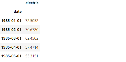
Read the Electric_Production dataset
#Read the Electric_Production dataset
Electric_Production = pd.read_csv('Electric_Production.csv', index_col ='date', parse_dates = True)

#Print the first five rows of the dataset
Electric_Production.head(5)
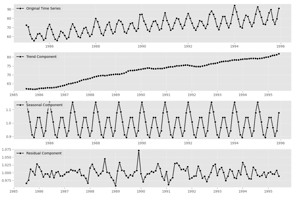
Assuming ‘Electric_Production’, original time series, Trend, Seasonal, Residual component
from statsmodels.tsa.seasonal import seasonal_decompose
import matplotlib.pyplot as plt

# Assuming 'Electric_Production' is your original time series data
result = seasonal_decompose(Electric_Production['electric'], model='multiplicative')

# Plotting the ETS decomposition with custom colors
plt.figure(figsize=(12, 8))

# Original time series
plt.subplot(411)
plt.plot(Electric_Production['electric'], label='Original Time Series', color='black', linestyle='-',marker='o', markerfacecolor='black', markeredgecolor='white')
plt.legend(loc='upper left')
plt.grid(True, linestyle='--', alpha=0.7)

# Trend component
plt.subplot(412)
plt.plot(result.trend, label='Trend Component', color='black', linestyle='-',marker='o', markerfacecolor='black', markeredgecolor='white' )

plt.legend(loc='upper left')
plt.grid(True, linestyle='--', alpha=0.7)

# Seasonal component
plt.subplot(413)
plt.plot(result.seasonal, label='Seasonal Component', color='black', linestyle='-', marker='o', markerfacecolor='black', markeredgecolor='white')
plt.legend(loc='upper left')
plt.grid(True, linestyle='--', alpha=0.7)

# Residual component
plt.subplot(414)
plt.plot(result.resid, label='Residual Component', color='black', linestyle='-', marker='o', markerfacecolor='black', markeredgecolor='white')
plt.legend(loc='upper left')

# Add gridlines
plt.grid(True, linestyle='--', alpha=0.7)

# Adjust layout
plt.tight_layout()


# Display the plot
plt.show()
# Import the library
from pmdarima import auto_arima

# Ignore harmless warnings
import warnings
warnings.filterwarnings("ignore")
Fit Auto ARIMA
stepwise_fit = auto_arima(Electric_Production,
                           start_p=1,  # Starting value of the autoregressive (AR) component
                           start_q=1,  # Starting value of the moving average (MA) component
                           max_p=3,    # Maximum value of the AR component
                           max_q=3,    # Maximum value of the MA component
                           m=12,       # Number of periods in each season (assuming monthly data)
                           start_P=0,  # Starting value of the seasonal AR component
                           seasonal=True,  # Indicates whether the data has a seasonal pattern
                           d=None,     # Order of differencing for the non-seasonal component (automatically determined)
                           D=1,        # Order of differencing for the seasonal component
                           trace=True,  # Prints debugging information during the fitting process
                           error_action='ignore',  # Determines how errors during fitting are handled
                           suppress_warnings=True,  # Suppresses convergence warnings
                           stepwise=True  # Uses a stepwise approach for model selection
                           )

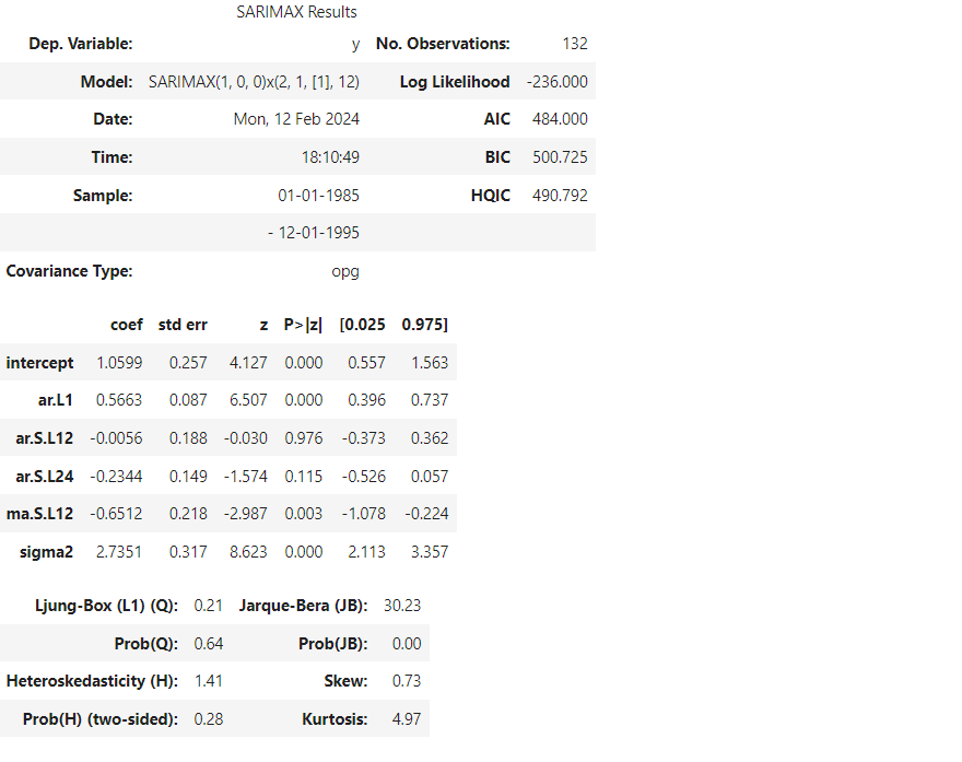
Summary of SARIMAX Results
# To print the summary
stepwise_fit.summary()
Split, train / test data
# Split data into train / test sets
train = Electric_Production.iloc[:len(Electric_Production)-12]
test = Electric_Production.iloc[len(Electric_Production)-12:] # set one year(12 months) for testing

# Fit a SARIMAX(0, 1, 1)x(2, 1, 1, 12) on the training set
from statsmodels.tsa.statespace.sarimax import SARIMAX

model = SARIMAX(train['electric'],
				order = (1, 0, 0),
				seasonal_order =(2, 1, 1, 12))

result = model.fit()
result.summary()

Generate diagnostic plots
# Generate diagnostic plots
result.plot_diagnostics(figsize=(12, 8))

# Save the plot to a file

plt.show()

Predictions for one year against the test set
start = len(train)
end = len(train) + len(test) - 1

# Predictions for one-year against the test set
predictions = result.predict(start, end, typ = 'levels').rename("Predictions")

# Visualize predictions vs actual values
plt.figure(figsize=(10, 6))

plt.plot(test['electric'], label='Actual Values', color='black', linestyle='-',
         marker='o', markerfacecolor='black', markeredgecolor='white')

plt.plot(predictions, label='Predictions', color='blue', linestyle='--',
         marker='o', markerfacecolor='blue', markeredgecolor='white')

plt.title('ARIMA forecasting Model: Actual vs Predicted')
plt.xlabel('Date')
plt.ylabel('Electric Production')
plt.legend(loc='upper right') # upper left

plt.savefig('arima forecasting model - actual vs predicted.png')
plt.show()

Assuming ‘test’ is your actual values and ‘predictions’ is the predicted values
Calculate evaluation metrics
Display the evaluation metrics
# Assuming 'test' is your actual values and 'predictions' is the predicted values
from sklearn.metrics import mean_absolute_error, mean_squared_error
import numpy as np
import matplotlib.pyplot as plt
from statsmodels.tsa.stattools import acf, pacf
from statsmodels.graphics.tsaplots import plot_acf, plot_pacf

# Calculate evaluation metrics
mae = mean_absolute_error(test['electric'], predictions)
mse = mean_squared_error(test['electric'], predictions)
rmse = np.sqrt(mse)

# Display the evaluation metrics
print(f'Mean Absolute Error (MAE): {mae:.2f}')
print(f'Mean Squared Error (MSE): {mse:.2f}')
print(f'Root Mean Squared Error (RMSE): {rmse:.2f}')

Train the model on the full dataset
# Train the model on the full dataset
model = model = SARIMAX(Electric_Production['electric'],
						order = (1, 0, 0),
						seasonal_order =(2, 1, 1, 12))
result = model.fit()
Forecast for the next 3 years
# Forecast for the next 3 years
forecast = result.predict(start = len(Electric_Production),
						end = (len(Electric_Production)-1) + 3 * 12,
						typ = 'levels').rename('Forecast')
print(forecast)

Arima forecasting values and confidence intervals
# Train the model on the full dataset
model = SARIMAX(Electric_Production['electric'],
                order=(1, 0, 0),
                seasonal_order=(2, 1, 1, 12))
result = model.fit()

# Forecast for the next 3 years
forecast = result.get_forecast(steps= 3 * 12)  # Forecast for the next 1 or 3 years 0r 5 years

# Extracting forecasted values and confidence intervals
forecast_values = forecast.predicted_mean.rename('Forecast')
ci_values = forecast.conf_int(alpha=0.05)  # 95% confidence interval

# Creating a DataFrame with forecast values and confidence intervals
forecast_df = pd.concat([forecast_values, ci_values], axis=1)
# Display the DataFrame
print(forecast_df)

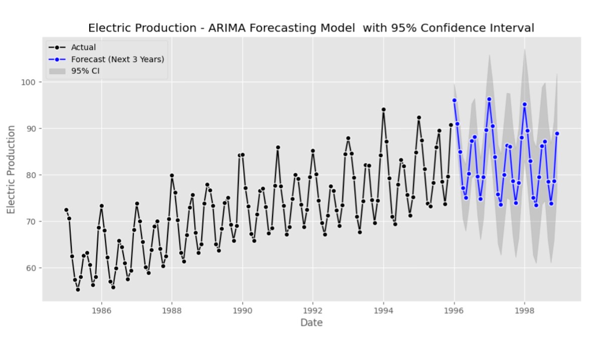
Electric Production – ARIMA Forecasting Model with 95% Confidence Interval
# Plotting the actual values, forecast, and confidence interval
plt.figure(figsize=(12, 6))

# Plot actual values
plt.plot(Electric_Production['electric'], label='Actual', color='blue')

# Plot forecast
plt.plot(forecast_values.index, forecast_values.values, label='Forecast', color='orange')

# Plot confidence interval
plt.fill_between(ci_values.index, ci_values.iloc[:, 0], ci_values.iloc[:, 1], color='orange', alpha=0.2, label='95% CI')

# Set plot labels and title
plt.title( 'Electric Production - ARIMA Forecasting Model  with 95% Confidence Interval')
plt.xlabel('Date')
plt.ylabel('Electric Production')

# Customize legend
plt.legend(loc='upper left')

# Show the plot
plt.show()

Full detailed plot – Electric Production – ARIMA Forecasting Model with 95% Confidence Interval
# Plotting the actual values, forecast, and confidence interval
plt.figure(figsize=(12, 6))

# Plot actual values
plt.plot(Electric_Production['electric'], label='Actual', color='black', linestyle='-', marker='o', markerfacecolor='black', markeredgecolor='white')

# Plot forecast
plt.plot(forecast_values.index, forecast_values.values,
         label='Forecast ( Next 3 Years)', color='green', linestyle='-', marker='o', markerfacecolor='green', markeredgecolor='white')

# Plot confidence interval
plt.fill_between(ci_values.index, ci_values.iloc[:, 0], ci_values.iloc[:, 1], color='gray', alpha=0.3, label='95% CI')

# Set plot labels and title
plt.title( 'Electric Production - ARIMA Forecasting Model  with 95% Confidence Interval')
plt.xlabel('Date')
plt.ylabel('Electric Production')

# Customize legend
plt.legend(loc='upper left')
plt.savefig('arima forecasting model_2.png')
# Show the plot
plt.show()
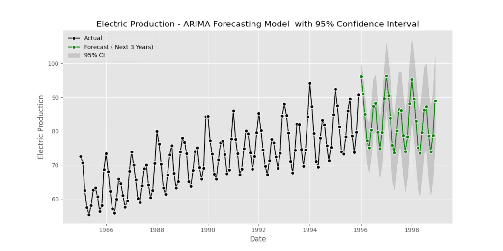
ARIMA forecasting model and having a solid understanding of time series analysis, businesses can harness the power of data analytics to predict future trends and gain a competitive advantage.
