Table of Contents
Introduction to Linear Regression
Linear regression in machine learning Python, a cornerstone concept in the fields of machine learning and statistical modeling, lays the foundation for understanding relationships between variables. Estimating the linear relationship between a dependent variable and one or more independent variables offers valuable insights into how changes in one variable affect another. This technique’s simplicity and interpretability make it a go-to choice for analyzing data and making predictions in various domains.
In machine learning, linear regression plays a vital role in predictive modeling tasks, where its ability to capture linear trends in data proves invaluable. Whether forecasting stock prices, predicting customer churn, or estimating housing prices, linear regression provides a solid framework for building predictive models.
Moreover, linear regression serves as a starting point for more advanced modeling techniques. Techniques like polynomial regression, ridge regression, and lasso regression are extensions of linear regression that address specific challenges such as overfitting and multicollinearity. Thus, mastering linear regression opens doors to understanding complex modeling approaches and enhances one’s ability to tackle real-world problems effectively.
In summary, linear regression’s significance must be balanced in the realm of machine learning and statistical modeling. Its simplicity, interpretability, and versatility make it an indispensable tool for data analysis, predictive modeling, and gaining insights into relationships between variables.
Understanding the Concept of Linear Regression in Machine Learning Python
Exploring Linear Regression in Machine Learning Python is an essential endeavor for anyone venturing into the realm of data analysis and predictive modeling. Leveraging Python’s robust libraries and tools, such as NumPy, Pandas, and Scikit-Learn, allows practitioners to seamlessly implement Linear Regression models with ease and efficiency. By understanding the foundational principles of Linear Regression and its practical application within the Python ecosystem, individuals can gain valuable insights into data relationships and make informed decisions. Whether forecasting future trends, optimizing business processes, or understanding complex phenomena, mastering Linear Regression in Machine Learning using Python empowers users to extract actionable intelligence from their data and drive meaningful outcomes.
Understanding Assumptions in Linear Regression
Linearity
The assumption of linearity states that there exists a linear relationship between the independent variables and the dependent variable. In other words, the change in the dependent variable is proportional to the change in the independent variables.
Independence of Errors
This assumption requires that the errors (residuals) between observed and predicted values are independent of each other. If errors are correlated, it can lead to biased estimates and inaccurate predictions.
Homoscedasticity
Homoscedasticity refers to the assumption that the variance of errors is constant across all levels of the independent variables. Violations of this assumption can lead to heteroscedasticity, where the spread of errors varies systematically.
Normality of Errors
The assumption of normality states that the errors follow a normal distribution with a mean of zero. Deviation from the norm can impact the trustworthiness of statistical tests and the accuracy of confidence intervals.
Importance of Assumptions in Linear Regression
It is imperative to grasp and confirm these assumptions to guarantee the reliability and accuracy of the linear regression model. Ignoring or violating these assumptions can lead to biased estimates, unreliable predictions, and incorrect inferences.
Checking Assumptions in Python
In Python, we can use various techniques to check the assumptions of linear regression.
Data Preparation First, ensure that the data is prepared properly, including handling missing values, encoding categorical variables, and scaling numerical features if necessary.
Scatterplots for Linearity
Visual inspection of scatterplots between independent and dependent variables can help assess the linearity assumption. A scatterplot should exhibit a clear linear pattern.

Residual Plots for Homoscedasticity
Plotting residuals against predicted values can help diagnose homoscedasticity. Ideally, the residuals should be randomly scattered around zero without any clear patterns.

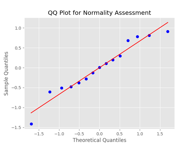
QQ Plots for Normality
QQ plots can be used to assess the normality of errors by comparing the distribution of residuals to a theoretical normal distribution. A straight diagonal line indicates normality

Simple Linear Regression
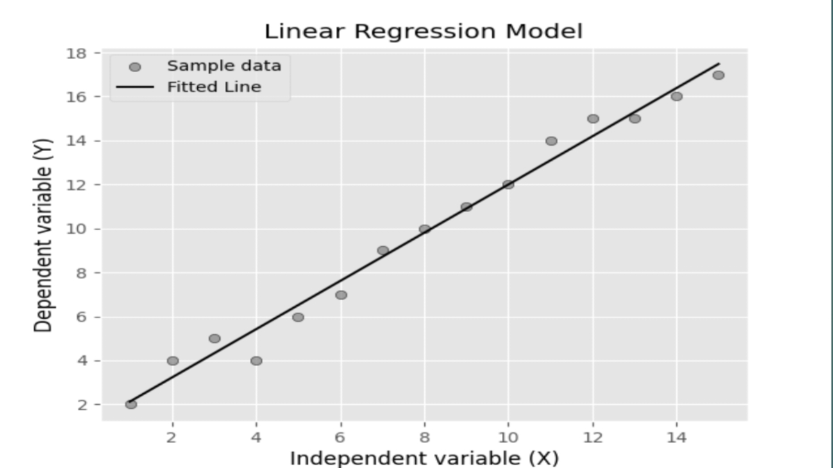
Simple linear regression involves a single independent variable. It is used when there is a linear relationship between the input and output variables. For instance, predicting house prices based on the area of the house is an example of simple linear regression. However, it’s essential to note the assumptions and limitations associated with this model, such as linearity, homoscedasticity, and independence of errors.
Simple Linear Regression in Machine Learning Python code example
simple linear regression model using the Ordinary Least Squares (OLS) method from the Statsmodels library
Import Libraries
import numpy as np
import pandas as pd
import matplotlib.pyplot as plt
import statsmodels.api as sm
Created Sample Data
X = np.array([1, 2, 3, 4, 5, 6, 7, 8, 9, 10,11,12,13,14,15])  # Independent variable
y = np.array([2, 4, 5, 4, 6, 7, 9, 10, 11, 12,14,15,15,16,17])  # Dependent variable
Create DataFrame
data = pd.DataFrame({'X': X, 'y': y})
Perform Linear Regression using the OLS model
X = sm.add_constant(X)  # Add constant term to the independent variable
model = sm.OLS(y, X).fit()
Print Model Summary
print(model.summary())

Multiple Linear Regression
Multiple linear regression extends the concept to include multiple independent variables. This allows for more complex modeling scenarios where the output depends on several factors simultaneously. For example, predicting stock prices based on various economic indicators involves multiple linear regression.
Step-by-step Guide to Implementing Linear Regression in Machine Learning Python
1. Data Preprocessing: Clean and preprocess the dataset by handling missing values, encoding categorical variables, and scaling features if necessary.
2. Splitting Data: Divide the dataset into training and testing sets to evaluate the model’s performance accurately.
3. Training the Model: Use the training data to fit the linear regression model to learn the underlying patterns in the data.
Importance of Evaluating Linear Regression Models
Ensuring the dependability and precision of the linear regression model hinges on comprehending and verifying these assumptions. By understanding model performance, we can make informed decisions about deploying the model in real-world scenarios.
Key Metrics for Evaluating Linear Regression Models.
Mean Absolute Error (MAE)
The Mean Squared Error (MSE) computes the average of the squared variances between predicted and actual values. It provides a straightforward interpretation of the model’s performance.
Mean Squared Error (MSE)
The Mean Squared Error (MSE) determines the average of the squared variances between the predicted and observed values. It penalizes larger errors more heavily than MAE, making it sensitive to outliers.
Root Mean Squared Error (RMSE)
RMSE is the square root of the MSE and provides a measure of the spread of errors. It’s commonly used as a more interpretable alternative to MSE.
Implementing Model Evaluation in Linear regression in machine learning Python
To evaluate linear regression models in Python, we’ll follow these steps:
1. Importing necessary libraries: We’ll import libraries such as NumPy, pandas, and scikit-learn for data manipulation and modeling.
2. Loading and preparing the dataset: We’ll load the dataset into a pandas DataFrame and preprocess it as needed.
3. Splitting the data into training and testing sets: We’ll divide the dataset into training and testing sets to train the model on one set and evaluate its performance on another.
4. Training the linear regression model: We’ll use scikit-learn to train a linear regression model on the training data.
5. Evaluating the model performance: We’ll use MAE, MSE, and RMSE to assess how well the model performs on the testing data.
Interpreting Evaluation Metrics
Once we have the evaluation metrics, we’ll interpret them to gain insights into the model’s performance. Lower values of MAE, MSE, and RMSE indicate better performance, while higher values suggest poorer performance.
Visualizing Model Performance
Visualizing the model’s predictions against the actual values can provide further insights into its performance. We’ll use plots such as scatter plots and line plots to visualize the relationship between the predicted and actual values.
Dealing with Overfitting and Underfitting
Overfitting occurs when the model captures noise in the training data and performs poorly on unseen data. Alternatively, underfitting arises when the model lacks the complexity needed to adequately capture the underlying patterns present in the data. We’ll discuss techniques such as regularization and cross-validation to mitigate these issues.
Real-World Examples and Use Cases
Linear regression finds applications across various domains, such as:
Predicting House Prices: Using features like square footage, number of bedrooms, and location to predict house prices.
Forecasting Sales: Analyzing historical sales data along with marketing expenditures to forecast future sales.
Advantages and Disadvantages:
Advantages
Simplicity: Easy to understand and interpret.
Speed: Quick to train and make predictions.
Interpretability: Provides insights into the relationship between variables.
Disadvantages
Assumptions: This relies on several assumptions that might not always hold.
Limited Complexity: This may not capture complex relationships between variables.
Sensitivity to Outliers: Outliers can significantly impact the model’s performance.
Conclusion
In conclusion, understanding and validating assumptions in linear regression are essential steps in building reliable predictive models. By ensuring that the data meets these assumptions, we can improve the accuracy and interpretability of our models. Linear regression serves as a foundational technique in machine learning, offering a simple yet powerful approach to modeling relationships between variables. By understanding its principles and implementing it in Python, practitioners can leverage its capabilities for predictive analytics and decision-making. Evaluating model performance is essential for building robust and reliable machine-learning models. By understanding key evaluation metrics and techniques, we can ensure that our linear regression models generalize well to new data and make accurate predictions in real-world applications.
Frequently Asked Questions
1. Is linear regression the same as correlation? No, although both deal with relationships between variables, correlation measures the strength and direction of the relationship, while linear regression models the relationship and predicts outcomes.
2. Can linear regression handle categorical variables? Yes, categorical variables can be encoded and included in a linear regression model, but they need to be properly handled through techniques like one-hot encoding.
3. What if the relationship between variables is not linear? In such cases, linear regression might not be the appropriate model. Techniques like polynomial regression or other nonlinear models can be considered.
4. How can we deal with multicollinearity in multiple linear regression? Multicollinearity, where independent variables are highly correlated, can be addressed by techniques like feature selection, regularization, or principal component analysis (PCA).
5. What is homoscedasticity, and why is it important? Homoscedasticity refers to the constant variance of errors across all levels of independent variables, and it’s important to ensure the reliability of model predictions.
6. What is the difference between MAE, MSE, and RMSE? The Mean Absolute Error (MAE) quantifies the average absolute variance between predicted and actual values, while the Mean Squared Error (MSE) computes the average squared variance between them. Root Mean Squared Error (RMSE), as the square root of MSE, offers a more understandable metric for error assessment.
7. How do you interpret evaluation metrics in linear regression? Superior model performance is indicated by lower values of MAE, MSE, and RMSE. Higher values suggest poorer performance and may indicate issues such as underfitting or overfitting.
8. What are some common techniques for dealing with overfitting and underfitting in linear regression? Methods for regularization, such as Lasso and Ridge regression, are commonly employed in statistical modeling. Cross-validation to assess model performance on unseen data.
9. Why is it important to visualize model performance? Visualizing model predictions helps to understand how well the model captures the underlying patterns in the data. It provides insights into areas where the model may be performing well or poorly.
10. How can I implement model evaluation in Python? You can use libraries such as scikit-learn to train linear regression models and evaluate their performance using metrics like MAE, MSE, and RMSE.
Read more
